AFNI version info (afni -ver): Precompiled binary linux_openmp_64: Sep 11 2024 (Version AFNI_24.2.06 'Macrinus')
Dear AFNI experts,
I am doing an HRF analysis on data that we collected awhile ago and described in this post.
Here is a summary:
- Patients or healthy controls
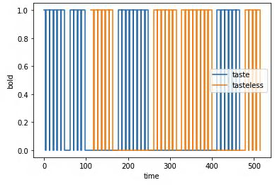
- Within-group design where each group receives a block of repeated taste or control stimulation according to a random choice of 4 pre-defined protocols (see below for an example of one protocols)

I did HRF estimation by running 3dDeconvolve on each subject to obtain stats_output+tlrc for each subject with 9 TENT functions:
3dDeconvolve -input "$feat_dir/denoised_func_data_nonaggr2standard.nii.gz" \
            -mask "${FSLDIR}/data/standard/MNI152_T1_2mm_brain_mask.nii.gz"\
            -polort A \
            -num_stimts 19 \
            -stim_times 1 $taste_onsets 'TENT(0, 8, 9)' -stim_label 1 HRF_MsA_Block1 \
            -stim_times 2 $tasteless_onsets 'TENT(0, 8, 9)' -stim_label 2 HRF_TlsA_Block1 \
	    -stim_file 3 $feat_dir/mc_csf_confevs.txt'[0]' -stim_base 3 -stim_label 3 Nuisance1 \
    	    -stim_file 4 $feat_dir/mc_csf_confevs.txt'[1]' -stim_base 4 -stim_label 4 Nuisance2 \
	    -stim_file 5 $feat_dir/mc_csf_confevs.txt'[2]' -stim_base 5 -stim_label 5 Nuisance3 \
	    -stim_file 6 $feat_dir/mc_csf_confevs.txt'[3]' -stim_base 6 -stim_label 6 Nuisance4 \
	    -stim_file 7 $feat_dir/mc_csf_confevs.txt'[4]' -stim_base 7 -stim_label 7 Nuisance5 \
	    -stim_file 8 $feat_dir/mc_csf_confevs.txt'[5]' -stim_base 8 -stim_label 8 Nuisance6 \
	    -stim_file 9 $feat_dir/mc_csf_confevs.txt'[6]' -stim_base 9 -stim_label 9 Nuisance7 \
	    -stim_file 10 $feat_dir/mc_csf_confevs.txt'[7]' -stim_base 10 -stim_label 10 Nuisance8 \
	    -stim_file 11 $feat_dir/mc_csf_confevs.txt'[8]' -stim_base 11 -stim_label 11 Nuisance9 \
	    -stim_file 12 $feat_dir/mc_csf_confevs.txt'[9]' -stim_base 12 -stim_label 12 Nuisance10 \
	    -stim_file 13 $feat_dir/mc_csf_confevs.txt'[10]' -stim_base 13 -stim_label 13 Nuisance11 \
	    -stim_file 14 $feat_dir/mc_csf_confevs.txt'[11]' -stim_base 14 -stim_label 14 Nuisance12 \
	    -stim_file 15 $feat_dir/mc_csf_confevs.txt'[12]' -stim_base 15 -stim_label 15 Nuisance13 \
	    -stim_file 16 $feat_dir/mc_csf_confevs.txt'[13]' -stim_base 16 -stim_label 16 Nuisance14 \
	    -stim_file 17 $feat_dir/mc_csf_confevs.txt'[14]' -stim_base 17 -stim_label 17 Nuisance15 \
	    -stim_file 18 $feat_dir/mc_csf_confevs.txt'[15]' -stim_base 18 -stim_label 18 Nuisance16 \
	    -stim_file 19 $feat_dir/mc_csf_confevs.txt'[16]' -stim_base 19 -stim_label 19 Nuisance17 \
            -fout -tout -x1D "$output_dir/X.xmat.1D" -xjpeg "$output_dir/X.jpg" \
            -bucket "$output_dir/stats_output"
mc_csf_confevsare csf and motion correction nuisance variables
Then I computed the contrast between taste and tasteless for each subject by subtracting the appropriate sub-bricks using 3dcalc (I'm also not sure if this is what I'm supposed to do, so if this is wrong please let me know):
while IFS= read -r line || [[ -n "$line" ]]; do
	echo "starting"

	subjID=$(echo "$line" | awk '{print$1}')
	echo "Processing subjID: $subjID"


	# getting pain or control
	pain_condition=$(echo "$line" | awk '{print$4}')
	parent_directory="$base_directory"/"$pain_condition"

	subject_dir="$parent_directory"/${subjID}/ses-bsl/func/AFNI_preproc/run_concat
	echo "$parent_directory"
	echo "$subject_dir"


	counter=1
	for i in $(seq 1 2 17); do
		j=$((20+(i-1)))  # indices for tasteless
		# subtracting taste and tasteless
		3dcalc -a "$subject_dir"/stats_output+tlrc[${i}] -b "$subject_dir"/stats_output+tlrc[${j}] \
			-expr 'a-b' \
			-prefix "$subject_dir"/contrast_t${counter}

		counter=$((counter+1))
	done
Then I ran 3dMSS on the taste, tasteless, and contrast conditions. Here is the specification for the contrast model. The taste and tasteless specifications are similar.
3dMSS -prefix output_contrast -jobs 16 \
	-lme 's(TENT,k=9)+s(TENT,k=9,by=pain)' \
	-ranEff 'list(Subj=~1)' \
	-qVars 'pain,TENT' \
	-prediction @HRF.contrast.table \
	-dataTable @contrast_df2.tsv
Last I used 3dbucket again to get the beta values for each point along the HRF so I could plot them.
I am having a little bit of trouble interpreting the output. Here are some questions I have:
-
How do I find the chi-square statistic? The
3dMSSdocumentation seems to suggest that sub-brick #0 (labeled intercept) is the chi-square value (specifically: "In the output the first sub brick shows the statistical evidence in the form of chi square distribution with 2 degrees of freedom"). Is this right? -
What would be best way to report results? The chi-square across the brain? The s(TENT):pain interaction? Something else?
-
We hypothesized that we would find significant interactions in subcortical structures such as the nucleus accumbens. Would it be permissible to do a ROI analysis without doing FDR correction? If so, would it be better to re-do the 3dMSS using a different mask, or would the current results be sufficient?
-
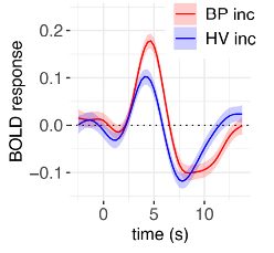
Is there any way to plot error bars in afni, like figure 6 in Chen et al. (2023)? Or would we have to take the mean/SE HRF within an ROI and then plot with other software?

-
Can we correct for other covariates such as age, sex, or BMI?
Sorry for asking so many questions. Please let me know if any of this is unclear.
Thank you again for all your help.