Why do EPIs show obvious horizental variance lines?

AFNI version info (afni -ver): 23.3.14

Dear AFNI members:

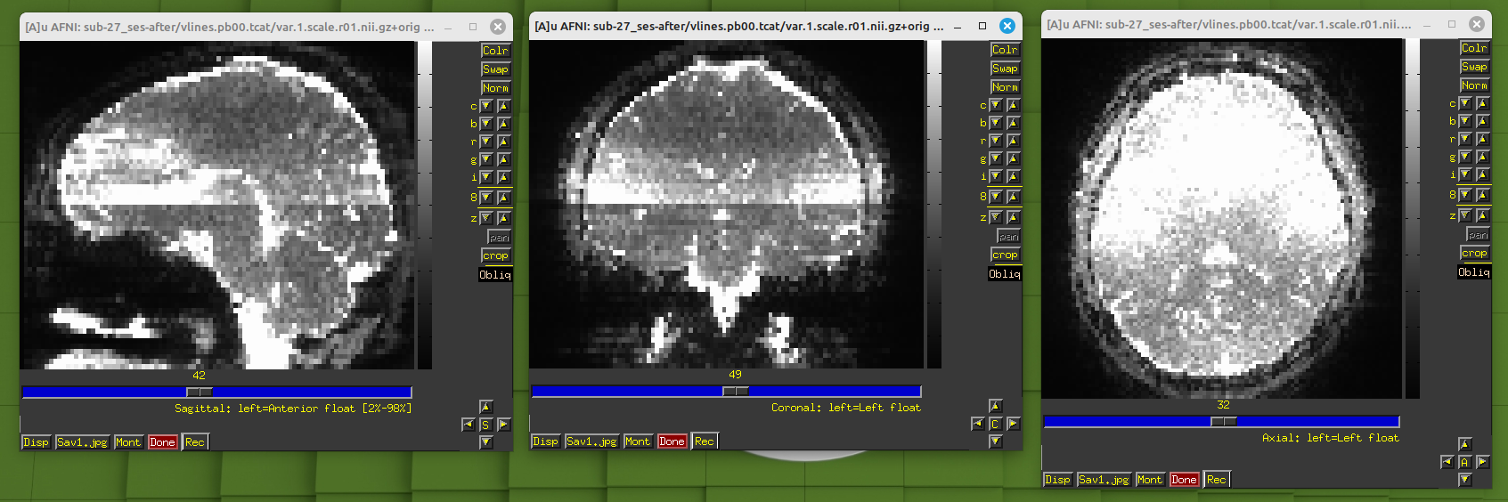
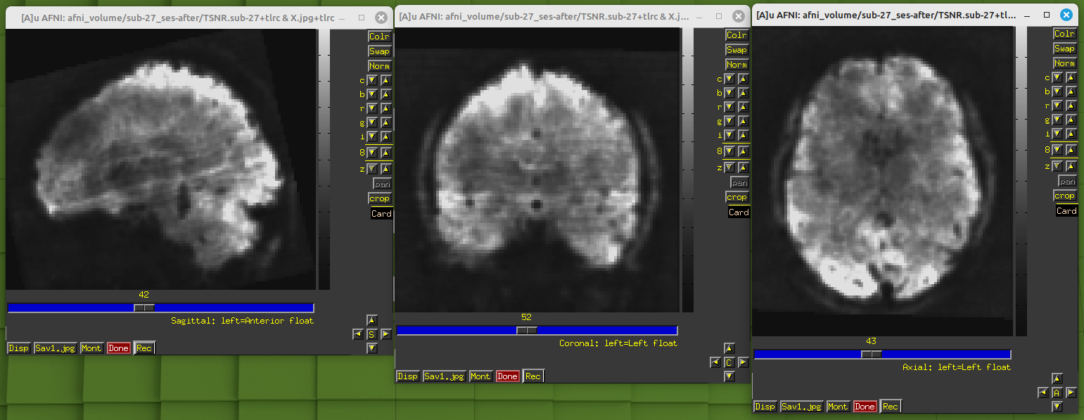
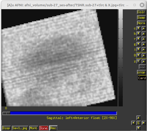
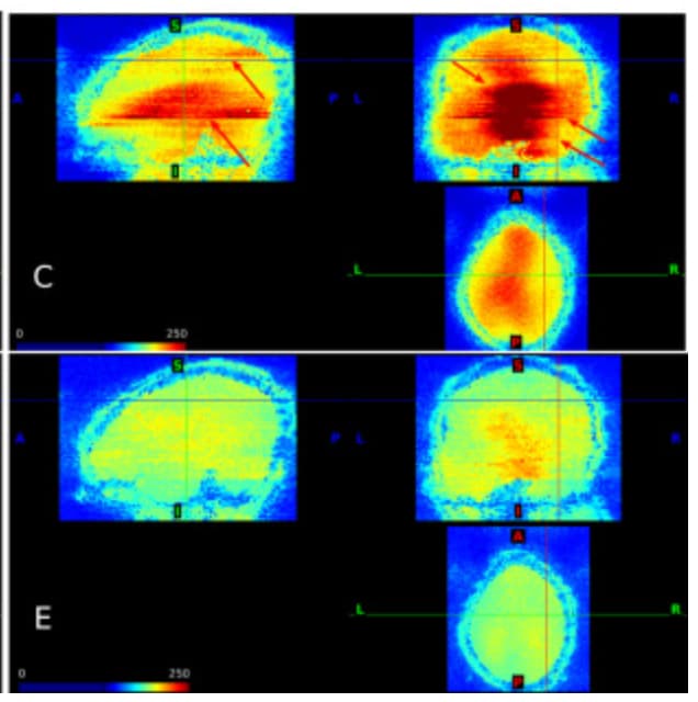
During the QC, I found my dataset shows obvious horizental variance lines though it indicates the vertical lines which are less obvious. I don't know how to explain it. I wonder whether this phenomenon correlates with some scan options, like phase encoding direction and whether this dataset is valuable to the following analysis.


PhaseEncodingDirection: J

How were the original slices acquired? Do they happen to be coronal images? There seems to be impressively little distortion.

  • rick

The slices were acquired from inferior to superior. These variance lines can be seen in coronal images too.

Okay, they are still axial slices. Maybe that is from a single large, sudden motion part way through the run. The dividing line might then show which slice was being acquired when the motion started. The vlines are computed on the original data, before motion correction.

What does that run's enorm look like?

  • rick

Considering that nearly all subjects in this dataset have this distortion, I think the main causes may be the scanner. I wonder whether this distortion will have any negative effects on the following functional connection analysis ( resting state ).

Is this multi-band EPI data?

If so, what MB factor, and what RF head coil are you using for acquiring these data?

1 Like

Yes. The multiband acceleration factor is 2. And if we see the slice timing, it seems that the variance lines is just at the beginning of the 2nd acquisition.
I can not provide more information about RF head coil at present.

Slice timing of this file (TR=2s, 64 TRs):
1.485, 0, 0.99, 0.0625, 1.0525, 0.125, 1.115, 0.185, 1.175, 0.2475, 1.2375, 0.31, 1.3, 0.3725, 1.3625, 0.4325, 1.4225, 0.5575, 1.5475, 0.62, 1.61, 0.68, 1.67, 0.7425, 1.7325, 0.805, 1.795, 0.8675, 1.8575, 0.9275, 1.9175, 0.495, 1.485, 0, 0.99, 0.0625, 1.0525, 0.125, 1.115, 0.185, 1.175, 0.2475, 1.2375, 0.31, 1.3, 0.3725, 1.3625, 0.4325, 1.4225, 0.5575, 1.5475, 0.62, 1.61, 0.68, 1.67, 0.7425, 1.7325, 0.805, 1.795, 0.8675, 1.8575, 0.9275, 1.9175, 0.495

Without information on the coil, we can only speculate. But from the variance patterns in your images, it seems that this coil's geometry does not support multi-band acquisition at all - at least along the head-foot axis of the subject.

Which parameters of RF head coil do I need to provide? In the BIDS json file, I can find some relevant keys. These may be useful:

"Manufacturer": "Siemens",
"ManufacturersModelName": "Prisma",
"ScanningSequence": "EP",
"SequenceVariant": "SK",
"ScanOptions": "FS",
"SequenceName": "*epfid2d1_94",
"ImageType": [
    "ORIGINAL",
    "PRIMARY",
    "FMRI",
    "NONE",
    "ND",
    "MOSAIC"
],
"NonlinearGradientCorrection": false,
"SeriesNumber": 12,
"SliceThickness": 2,
"SpacingBetweenSlices": 2.5,
"SAR": 0.0772278,
"EchoTime": 0.03,
"RepetitionTime": 2,
"FlipAngle": 80,
"PartialFourier": 1,
"BaseResolution": 94,
"ShimSetting": [
    -3199,
    -5816,
    -5702,
    254,
    26,
    -189,
    -127,
    -21
],
"TxRefAmp": 259.812,
"PhaseResolution": 1,
"ReceiveCoilName": "HeadNeck_20",
"ReceiveCoilActiveElements": "HE1-4;NE1,2",
"PulseSequenceDetails": "%SiemensSeq%\\ep2d_bold",
"RefLinesPE": 24,
"CoilCombinationMethod": "Sum of Squares",
"ConsistencyInfo": "N4_VE11C_LATEST_20160120",
"MultibandAccelerationFactor": 2,
"PercentPhaseFOV": 100,
"PercentSampling": 100,
"EchoTrainLength": 47,
"PhaseEncodingSteps": 94,
"AcquisitionMatrixPE": 94,
"ReconMatrixPE": 94,
"BandwidthPerPixelPhaseEncode": 40.145,
"ParallelReductionFactorInPlane": 2,
"EffectiveEchoSpacing": 0.000264997,
"DerivedVendorReportedEchoSpacing": 0.000529994,
"TotalReadoutTime": 0.0246447,
"PixelBandwidth": 2315,
"DwellTime": 2.3e-06,
"PhaseEncodingDirection": "j",

Yes - that's sufficient. These data were acquired with Siemens' 20-channel head coil. You would need to make sure the geometry of that coil is adequate for SMS.

This link describes a bit what I think the issue might be here. This article describes the 12 and 32 Siemens head coils, but does not cover the 20.

hi all-

i spotted this thread and chatted with my colleague An (Joseph) Vu about it... he mentioned this older thread (he's "whitecraine") where it's suggested the RF pulse may be too short: banding artifact in BOLD std maps. (Prisma) · Issue #217 · CMRR-C2P/MB · GitHub hopefully this helps or lends more insight.

-sam

@storissi and @roopv have posted potential solutions for future acquisitions. If you're trying to figure out if the data you already have is good enough for analysis, you will want to look at some other images. What do the post-volreg TSNR images look like in your QC? The GCOR images? In the sagittal and coronal views, do you see lower SNR in the top than the bottom? Does the additional noise correlate so much they dominate the correlation you would see with InstaCorr? Are you doing a resting state or task based analysis?

1 Like

Sorry for the late reply.

Hi @roopv I find it's difficult for me to grasp the core information of that blog. But the author provides another info, which may partially explains this phenomenon. That is if the total number of slices divided by the MB factor is even (as for my dataset), the saturation artifacts will occur at the beginning of the 2nd acquisition (figure 3 in this paper).

Hi @storrisi Yes, it's helpful. These issues are very same to mine. Thanks.

Hi @dglen I am doing resting state analysis. I have re-checked the other QC images. The TSNR shows the same distortion from the coronal and sagittal views. The first slice in sagittal view shows parallel stripes covering the whole image. Because of deobliquity, the axial view shows little information. (The example images use the grayscale mode because color mode can interfere observations.)


image

I did not find more useful information from GCOR images or with InstaCorr (you know, I am a relative beginner). If some expert needs, I can provide raw data.

Hi @renyiyuan,

To me this looks like a common feature of thermal noise-limited protocols of Multi-band images. E.g with extreme acceleration, very high resolution, small flip angles, very short TRs, coil with low number of elements etc.
Example 1


from http://dx.doi.org/10.1016/j.neuroimage.2018.01.078 fig 2.

Example 2 https://youtu.be/kzh-nWXd54s?si=44tyGb6JM3J8H607&t=4849

I do not think there is anything wrong here from the acquisition side. While g-factors are expected to be smooth within slices (for commonly small GRAPPA kernels), it is not expected that g-factor noise amplification is smooth at the edges of multi-band slabs. It's just that the edge is usually hidden in the physiological noise. I think many people run their studies with similarly agressive protocols and with these edges in variance.
In general, with Multiband, one cannot (should not) assume that the noise is homogeneously, nor smoothly distributed in space. Since the head is not a square, the CAIPI unaliasing pattern will now homogeneously distribute across the FOV.
If your study is really limited by the edge of the variance maps, I think all the potential edits in the data acquisition have been mentioned incl.: using different RF coil, smaller MB factors, leak block recon, which will come with compromises.

Best regards, Renzo

1 Like

Hi @Renzo_Huber, thanks for your valuable reply. I will try to continue the functional connectivity analysis and be careful with this issue. And if I find any useful correlations between this artifacts and FC, I will report it here.

Howdy-

A useful thing to check when you process this resting state data are some the afni_proc.py QC HTML features, like the seed-based correlation, corr_brain, rad_cor and TSNR maps described here (see Figs. 4 and following):
https://www.frontiersin.org/articles/10.3389/fnins.2022.1073800/full
... and esp. the InstaCorr (IC) and Graph View (GV) buttons for quick, interactive surfing of the data, as described here:
https://afni.nimh.nih.gov/pub/dist/OHBM2023/ohbm_2023_apqc_html_taylor_etal.pdf

The simplest way to check this out on your data would be to have a modern AFNI version, and run the very simple set-up form of afni_proc.py that Rick created, so you don't need a lot of options (though, when you have your real analysis, controlling all the options is highly useful!) just the dset names and subject ID:

ap_run_simple_rest.tcsh                                                      \
    -epi       DSET_EPI                                                      \
    -anat      DSET_ANAT                                                     \
    -subjid    SUBJ_ID                                                       \
    -run_ap                                                                  \
    -run_proc

When that is done, open the APQC report with the local server running (requires Flask and Flask-Cors Python modules to be present, which are now part of the AFNI system setup):

open_apqc.py -infiles path_to_results_dir/QC_*/index.html

Look at the seedbased correlation maps, TSNR, corr_brain and radcor, and the IC and GV buttons above those images will let you run InstaCorr and the Graph View QCs quickly.

--pt

Oh, and looking more closely at your thread images, I see you are running afni_proc.py already...

The GV, IC and other buttons are "greened" out above the images, meaning that they were not opened with the local server running. Let me know if you need any assistance with that aspect.

--pt