Partitioning shared variance among predictors

[Gang]

Partitioning shared variance among predictors

Gang Chen

In statistical modeling, it is sometimes valuable to dissect the variance of a response variable among multiple predictors. A key metric for this purpose is the coefficient of determination, denoted as R^2. This metric quantifies the proportion of variability in the response variable that can be attributed to one or more predictors. For a comprehensive understanding of its definition and practical applications, refer to the Wikipedia page.

In this specific context, we derive the partitioning of R^2 when dealing with two or three predictors. Our approach draws inspiration from a tutorial by Peter E. Kennedy, which employs Venn diagrams for visual representation during derivation.

Three variables: x, y and h

Suppose a regression model for the response variable h is constructed with x and y as two predictors. Assume that R_{x(x)}^2 and R_{y(y)}^2 are the coefficients of determination for the models h\sim x and h\sim y (using the Wilkinson notation), respectively, while R_{x(xy)}^2 and R_{y(xy)}^2 are the coefficients of partial determination for the model h\sim x+ y. In other orders, the four coefficients of determination are associated with the following three models:

\begin{aligned} R_{x(x)}^2:&~h\sim x,\\ R_{y(y)}^2:&~h\sim y,\\ R_{x(xy)}^2,R_{y(xy)}^2:&~h\sim x+y. \end{aligned}

Assume that the unique proportion of variability that variable x accounts for in h is q_x. Similarly, the unique proportion of variability that variable y contributes to z is q_y. Lastly, the shared (or common) proportion of variability that variables x and y contribute together to h is q_{xy}. These three proportions can conceptually represented by the following Venn diagram:


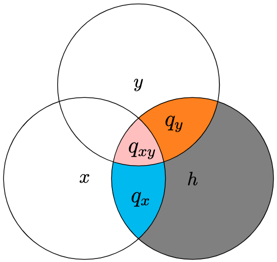
The above pictorial representation intuitively results in the following relationships:

\begin{aligned} q_x+q_{xy}&=R_{x(x)}^2,\\ q_y+q_{xy}&=R_{y(y)}^2,\\ q_x+q_{xy}+q_y&=R_{x(xy)}^2+R_{y(xy)}^2.\\ \end{aligned}

Solving the above simultaneous equations leads to

\begin{aligned} q_x=&(R_{x(xy)}^2+R_{y(xy)}^2)-R_{y(y)}^2,\\ q_y=&(R_{x(xy)}^2+R_{y(xy)}^2)-R_{x(x)}^2,\\ q_{xy}=&(R_{x(x)}^2+R_{y(y)}^2)-(R_{x(xy)}^2+R_{y(xy)}^2). \end{aligned}

Four variables: x, y, z and h

Suppose a regression model for the response variable h is constructed with x, y and z as three predictors. Following the same notation convention as the case with three variables above, we associate twelve coefficients of determination with the following seven models:

\begin{aligned} R_{x(x)}^2: &~h\sim x,\\ R_{y(y)}^2: &~h\sim y,\\ R_{z(z)}^2: &~h\sim z,\\ R_{x(xy)}^2, R_{y(xy)}^2: &~h\sim x+y,\\ R_{x(xz)}^2, R_{z(xz)}^2: &~h\sim x+z,\\ R_{y(yz)}^2, R_{z(yz)}^2: &~h\sim y+z,\\ R_{x(xyz)}^2, R_{y(xyz)}^2, R_{z(xyz)}^2: &~h\sim x+y+z. \end{aligned}

There are seven partitioned proportions of variability that are of interest in this case. Assume that the unique proportions of variability that variables x, y and z account for in h are q_x, q_y and q_z. Similarly, the shared proportion of variability that variables x and y contribute together to h is q_{xy}; the shared proportion of variability that variables x and z contribute together to h is q_{xz}; the shared proportion of variability that variables y and z contribute together to h is q_{yz}. Lastly, the shared proportion of variability that variables x, y and z contribute together to h is q_{xyz}.

These seven proportions likely lend themselves to a graphic representation through a Venn diagram, although I haven’t yet crafted an elegant one. If you have any brilliant suggestions, please don’t hesitate to share! Nonetheless, deriving the following relationships isn’t particularly challenging:

\begin{aligned} q_x+q_{xy}+q_{xz}+q_{xyz}&=R_{x(x)}^2,\\ q_y+q_{xy}+q_{yz}+q_{xyz}&=R_{y(y)}^2,\\ q_z+q_{xz}+q_{yz}+q_{xyz}&=R_{z(z)}^2,\\ q_x+q_y+q_{xy}+q_{yz}+q_{xz}+q_{xyz}&=R_{x(xy)}^2+R_{y(xy)}^2,\\ q_x+q_z+q_{xy}+q_{yz}+q_{xz}+q_{xyz}&=R_{x(xz)}^2+R_{z(xz)}^2,\\ q_y+q_z+q_{xy}+q_{yz}+q_{xz}+q_{xyz}&=R_{y(yz)}^2+R_{z(yz)}^2,\\ q_x+q_y+q_z+q_{xy}+q_{yz}+q_{xz}+q_{xyz}&=R_{x(xyz)}^2+R_{y(xyz)}^2+R_{z(xyz)}^2. \end{aligned}

Despite its tedium, algebra can assist in deciphering the equations above and yield the following solutions for the seven partitioning components.

\begin{aligned} q_x=&(R_{x(xyz)}^2+R_{y(xyz)}^2+R_{z(xyz)}^2) - (R_{y(yz)}^2+R_{z(yz)}^2),\\ q_y=&(R_{x(xyz)}^2+R_{y(xyz)}^2+R_{z(xyz)}^2) - (R_{x(xz)}^2+R_{z(xz)}^2),\\ q_z=&(R_{x(xyz)}^2+R_{y(xyz)}^2+R_{z(xyz)}^2) - (R_{x(xy)}^2+R_{y(xy)}^2),\\ q_{xy}=&(R_{x(xz)}^2+R_{z(xz)}^2)+(R_{y(yz)}^2+R_{z(yz)}^2)-R_{z(z)}^2-(R_{x(xyz)}^2+R_{y(xyz)}^2+R_{z(xyz)}^2),\\ q_{xz}=&(R_{x(xy)}^2+R_{y(xy)}^2)+(R_{y(yz)}^2+R_{z(yz)}^2)-R_{y(y)}^2-(R_{x(xyz)}^2+R_{y(xyz)}^2+R_{z(xyz)}^2),\\ q_{yz}=&(R_{x(xy)}^2+R_{y(xy)}^2)+(R_{x(xz)}^2+R_{z(xz)}^2)-R_{x(x)}^2-(R_{x(xyz)}^2+R_{y(xyz)}^2+R_{z(xyz)}^2),\\ q_{xyz}=&R_{x(x)}^2+R_{y(y)}^2+R_{z(z)}^2+(R_{x(xyz)}^2+R_{y(xyz)}^2+R_{z(xyz)}^2)-(R_{x(xy)}^2+R_{y(xy)}^2)-(R_{x(xz)}^2+R_{z(xz)}^2)-(R_{y(yz)}^2+R_{z(yz)}^2). \end{aligned}

Notice that the coefficients of determination are grouped according to their associated models: those enclosed within a pair of parentheses () correspond to the same model.