Nonlinear Modeling
Gang Chen
Preface
Capturing nonlinear relationships is pivotal in statistical modeling. Linear models are widely embraced due to their familiarity, intuitive interpretation, mature toolset, and computational efficiency. However, understanding and incorporating nonlinearity is equally crucial. When a function f(x) is smooth enough at the point x_0, its Taylor expansion can be expressed as,
f(x)=f(x_0)+f'(x_0)(x-x_0)+\frac{1}{2}f''(x_0)(x-x_0)^2+...
This expansion indicates that the linear approximation of f(x) likely holds in the neighborhood of x_0. In other words, it might be essential to consider nonlinearity, especially when the range of x is relatively wide. For instance, brain development or BOLD response over a short period (i.e., 2-3 years) could be approximated as linear. Still, it's likely to demonstrate strong nonlinear relationships over a more extended period (e.g., adolescence).
Numerous methods can capture nonlinearity in data. If prior information is available, a specific functional form or variable transformation can be adopted. However, when prior knowledge is lacking, addressing nonlinearity conventionally involves using polynomial fitting. Nevertheless, polynomial models present challenges such as non-locality, difficulties in order selection, and comparisons between curves.
-
Non-locality or instability: the fitted curve at a particular location may be sensitive to the data far from that point.
-
Order selection: It is difficult to predetermine the order of polynomial fitting, which is especially problematic with the heterogeneity across brain regions.
-
Difficulty in comparing two fitted curves: no simple statistical tools are available to make comparisons across fitted polynomials.
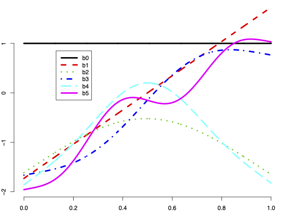
An effective alternative for capturing nonlinearity without prior knowledge is employing splines. One significant advantage of using splines for fitting is their adaptability: the model learns the relationship from the data while maintaining conservatism on excessive roughness. Etymologically referring to a thin strip used to draft smooth curves, splines offer versatile options, with piecewise cubic splines being popular. In this discussion, we introduce a special type: thin plate splines. Two unique features set them apart--each thin basis is not tied to a specific knot, and nonlinearity complexity grows incrementally with the number of bases. Specifically, the first two bases (represented by b_0 and b_1 in the figure below) capture the baseline and linear trend, respectively.
Modeling with splines offers a flexible approach for fitting nonlinear relationships. One significant advantage is that one does not need to know the specifics of nonlinearity a priori. The model can adaptively learn from and fit the data through a penalization strategy against roughness.
Here, we introduce two programs that fit nonlinear relationships using thin plate splines: 3dMSS can be adopted for voxel/node-wise analysis, while PTA is implemented for trend estimation at the region level and other scenarios such as profile estimation of layer fMRI data. The theoretical background is detailed in the following paper:
Chen, G., Nash, T.A., Cole, K.M., Kohn, P.D., Wei, S.-M., Gregory, M.D., Eisenberg, D.P., Cox, R.W., Berman, K.F., Shane Kippenhan, J., 2021. Beyond linearity in neuroimaging: Capturing nonlinear relationships with application to longitudinal studies. NeuroImage 233, 117891. DOI: 10.1016/j.neuroimage.2021.117891
Below, we demonstrate a few use cases of 3dMSS . The usage of PTA follows a similar specification interface.
(1) Estimating nonlinear trend for a single group
In this scenario, data are collected at specific points (e.g., space or time) for each individual. A cross-sectional study is one such case. Let us consider neuroimaging data available from participants with varying ages. The following example showcases capturing the nonlinear trend across ages.
3dMSS -prefix MSS -jobs 16                  \
      -mrr   's(age,k=10)'                  \
      -qVars 'age'                          \
      -prediction @pred.txt                 \
      -dataTable  @data.txt
The s() part under -mrr is used to specify various components of nonlinear fitting: the predictor age and the number of splines k=10. When the number of data points (e.g., age values) is less than 6, fitting a meaningful nonlinear trend isn't practical. With 6 to 9 data points, k can be chosen up to the number of data points.
Input information is provided through a table data.txt, which contains the following:
Subj   age   InputFile
S1      20       S1.nii
S2      18       S2.nii
...
Similarly, information for the predicted trend is provided through the data table pred.txt:
   label  age
age11   11
age12   12
age13   13
...
age18   18
age19   19
age20   20
    ...
For better visualization, one may increase the prediction resolution (e.g., every 0.25 years instead of 1).
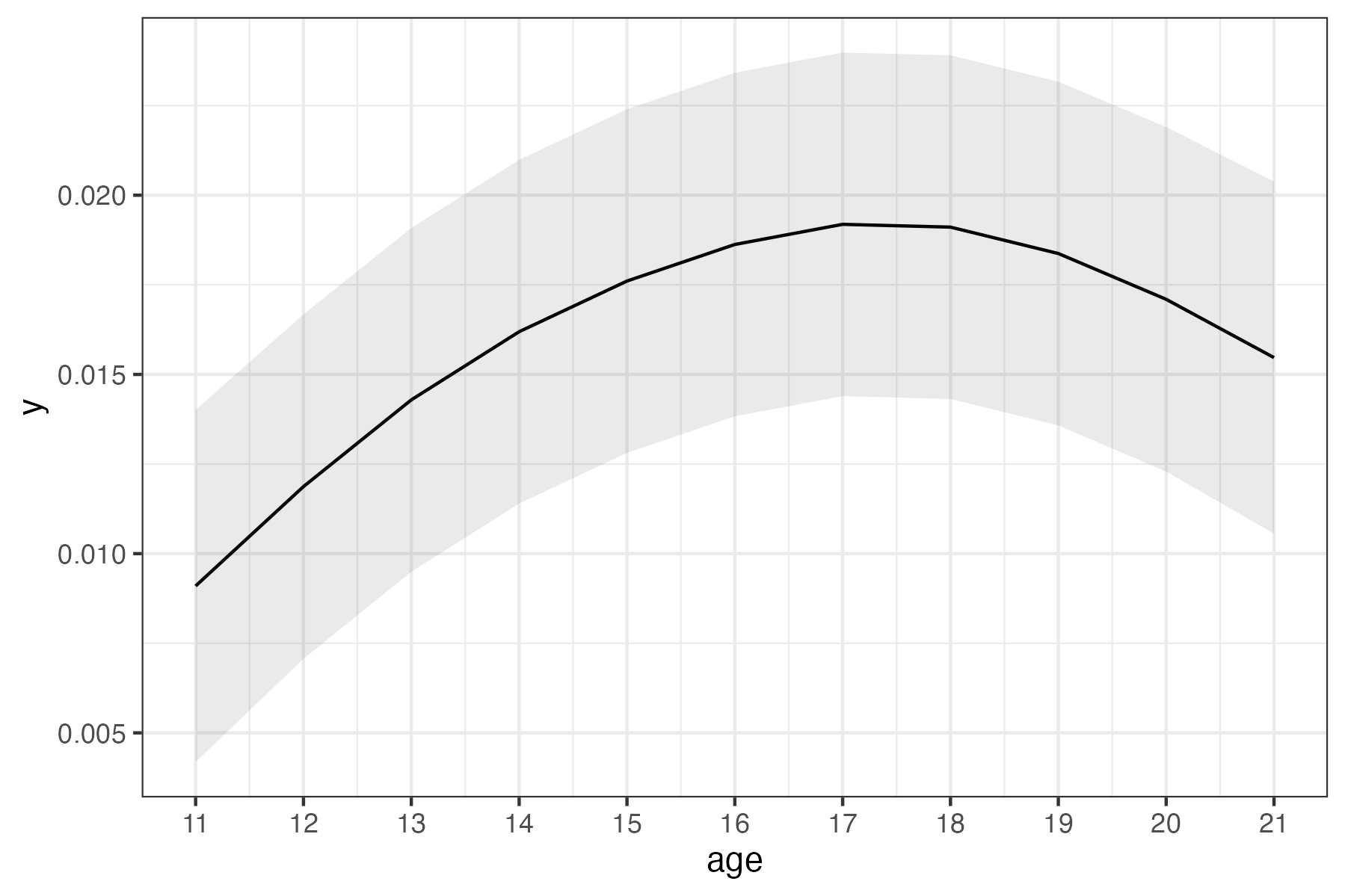
In the output, the sub-brick with a label containing s(age) shows the statistical evidence for the nonlinear trend. The predicted values in the output can be extracted (e.g., using 3dbucket) and visualized using the Graph button on the AFNI panel. One may plot them out (e.g., using R) at the voxel or region level, incorporating both the predicted values and their standard errors, as illustrated below:
If it is preferable to capture nonlinearity separate from the linear trend, replace the second line above with the following:
...
      -mrr 'age+s(age,k=10,m=c(2,0))'    \
...
The first part age captures the linear trend, and the second part s(age,k=10,m=c(2,0)) models the nonlinearity. In the output, the statistical evidence for the linear and nonlinear trends is separately labeled with age and s(age). The predicted trend should not change regardless of the linear trend being modeled separately.
(2) Comparing nonlinear trends between two or more groups
Suppose that we would like to compare the nonlinear trend between two groups. Quantitatively code the two groups with 1 and -1, and modify the 3dMSS script in the single group case above to the following:
3dMSS -prefix MSS -jobs 16                    \
      -mrr   's(age,k=10)+s(age,by=grp,k=10)' \
      -qVars 'age'                            \
      -prediction @pred.txt                   \
      -dataTable  @data.txt
The first component s(age,k=10) accounts for the average trend between the two groups while the second component s(age,by=grp,k=10) captures their difference.
The input information is similarly provided through a table data.txt except that the group column is coded with 1s and -1s:
Subj   age   grp  InputFile
S1      20    1    S1.nii
S2      18   -1    S2.nii
...
Similarly, the information for the predicted trend of each group is provided through the data table pred.txt:
   label     grp  age
g1.age11  1  11
g1.age12  1  12
g1.age13  1  13
...
g2.age11 -1  11
g2.age12 -1  12
g2.age13 -1  13
    ...
With more than two groups, the same strategy of deviation coding applies. Specifically, k groups requires k-1 columns in both the input and prediction tables.
(3) Estimating nonlinear trend of a single group with intra-individual data
In this scenario, data are collected at various points (e.g., in space or time) for each individual. A longitudinal study is a typical example of this case. Suppose neuroimaging data are available for each participant across a number of years. The following presents an example of capturing the nonlinear trend across different ages.
3dMSS -prefix MSS -jobs 16                  \
      -lme 's(age,k=10)'                    \
      -ranEff 'list(Subj=~1)'               \
      -qVars 'age'                          \
      -prediction @pred.txt                 \
      -dataTable  @data.txt
It's important to note that the population-level trend, denoted as 's(age,k=10)', is specified using the -lme option. Additionally, an extra component, -ranEff 'list(Subj=~1)', introduces an individual-specific shift, analogous to the concept of a random intercept in mixed-effects modeling.
(4) Comparing nonlinear trends between two conditions
In this scenario, data are collected at various points (e.g., in space or time) for each individual and are recorded under two distinct conditions at each point. For instance, in a longitudinal study, BOLD response is measured under both positive and negative conditions. Another example could involve estimating the elicited BOLD response or vascular space occupancy (VASO) across different cortex layers. These cases extend the scenario described in case (3) above, introducing an additional factor of condition or layer.
To effectively compare nonlinear trends, we recommend a data reduction approach. Begin by calculating the contrast between the two conditions at the individual level. Subsequently, utilize this contrast as input by following the procedure outlined in case (3) above.