AFNI version info (afni -ver):
Precompiled binary linux_ubuntu_16_64: May 23 2025 (Version AFNI_25.1.11 'Maximinus')
Hi,
I am trying to compare the motion parameters for a dataset processed with realtime afni and those obtained with just afni after converting data with dcm2niix.
The starting point is some data acquired with last year on our previous software platform Siemens VE11C, i.e. with good old Mosaic Dicoms (my aim at the end is to see compare these motions parameters the same way with the current software XA60 and enhanced DICOMs, but one step at a time).
Real time processing
first terminal window: realtime_receiver.py -show data yes
second terminal window:
setenv AFNI_REALTIME_Registration  3D:_realtime
setenv AFNI_REALTIME_Base_Image    0
setenv AFNI_REALTIME_Graph         Realtime
setenv AFNI_REALTIME_Resampling   cubic
setenv AFNI_REALTIME_MP_HOST_PORT  localhost:53214
...
setenv AFNI_REALTIME_SHOW_TIMES    YES
setenv AFNI_REALTIME_Mask_Vals     Motion_Only
setenv AFNI_REALTIME_Function 	   FIM
afni -rt -yesplugouts
followed by: Dimon -infile_prefix $pref -assume_dicom_mosaic -rt -quit
Offline processing
I start by converting the DICOMs with dcm2niix:
dcm2niix -o outputDir dicomDir
Then I run the following, which I am assuming is relatively close to what afni realtime afni does:
3dTcat -prefix pb00.tcat \
   outputDir/myfiles.nii'[0..$]'

3drefit -Tslices 1.110 0.000 0.740 0.062 0.803 0.125 0.865 0.185 0.925 0.248 0.988 0.310 1.050 0.433 1.173 0.495 1.235 0.555 1.295 0.618 1.358 0.680 1.420 0.370 1.110 0.000 0.740 0.062 0.803 0.125 0.865 0.185 0.925 0.248 0.988 0.310 1.050 0.433 1.173 0.495 1.235 0.555 1.295 0.618 1.358 0.680 1.420 0.370  pb00.tcat+orig

3dTshift -tzero 0 -quintic -prefix pb01.tshift \
             pb00.tcat+orig

3dvolreg -verbose -base 0                    \
             -1Dfile dfile.RT.1D -prefix pb01.volreg \
             -cubic                                                 \
		pb01.tshift+orig
I have also run the same script without 3drefit and 3dTshift, and called that curve "no Slice Ttiming".
I hope I was careful to notice that in realtime_receiver, the order of the output is
dS dL dP roll pitch yaw
while the order of the output file from 3dvolreg is:
roll pitch yaw dS dL dP
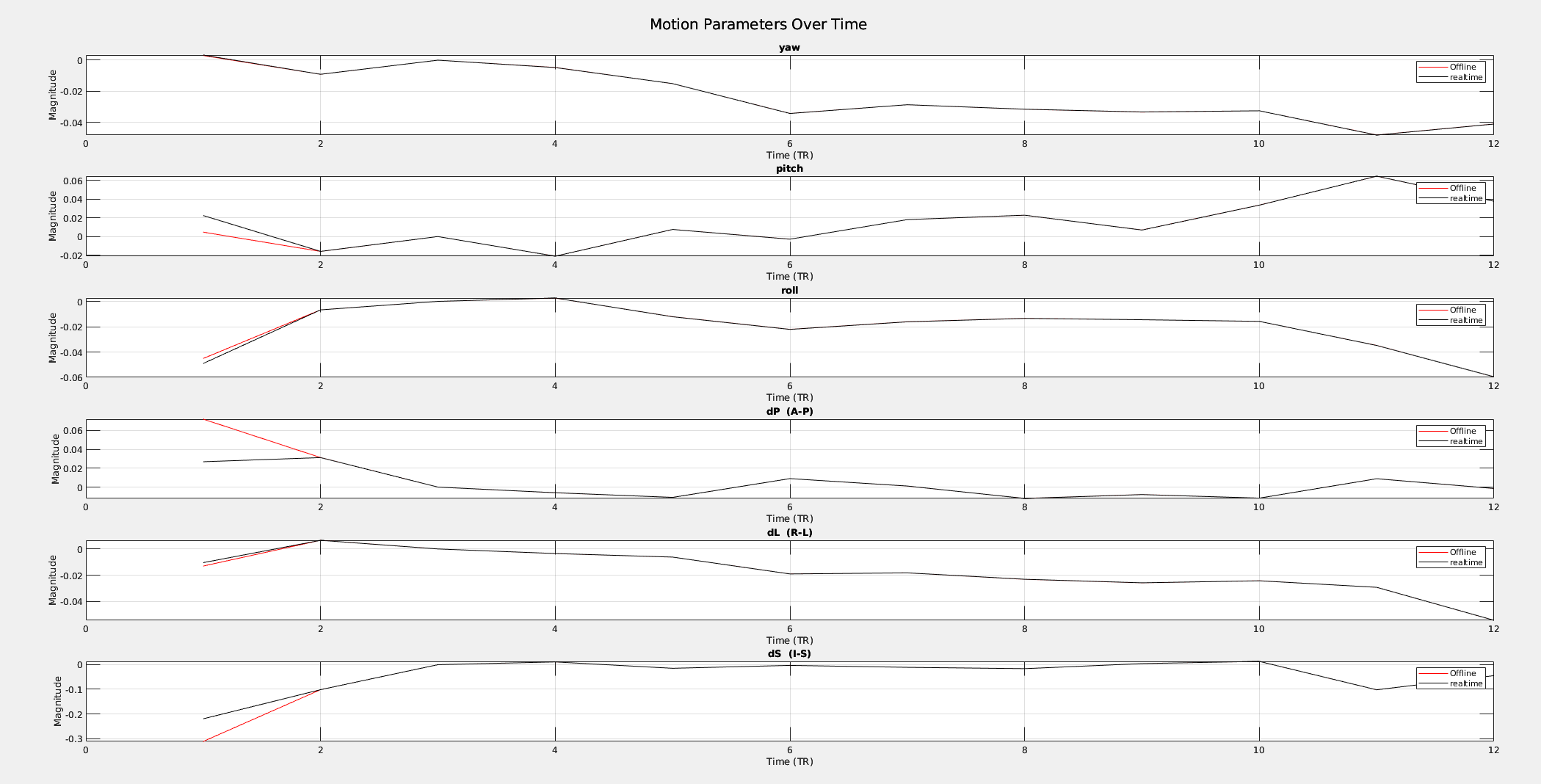
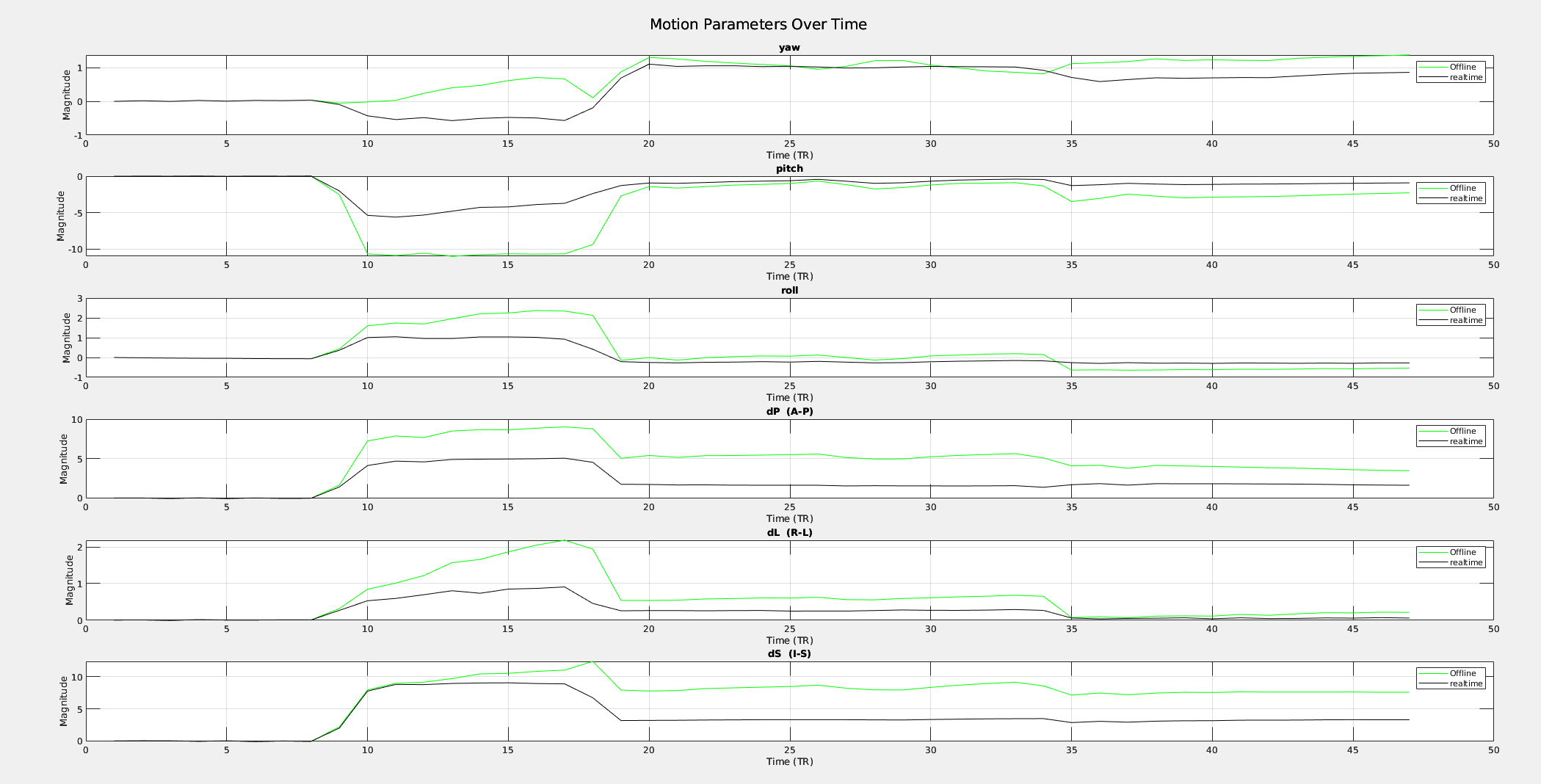
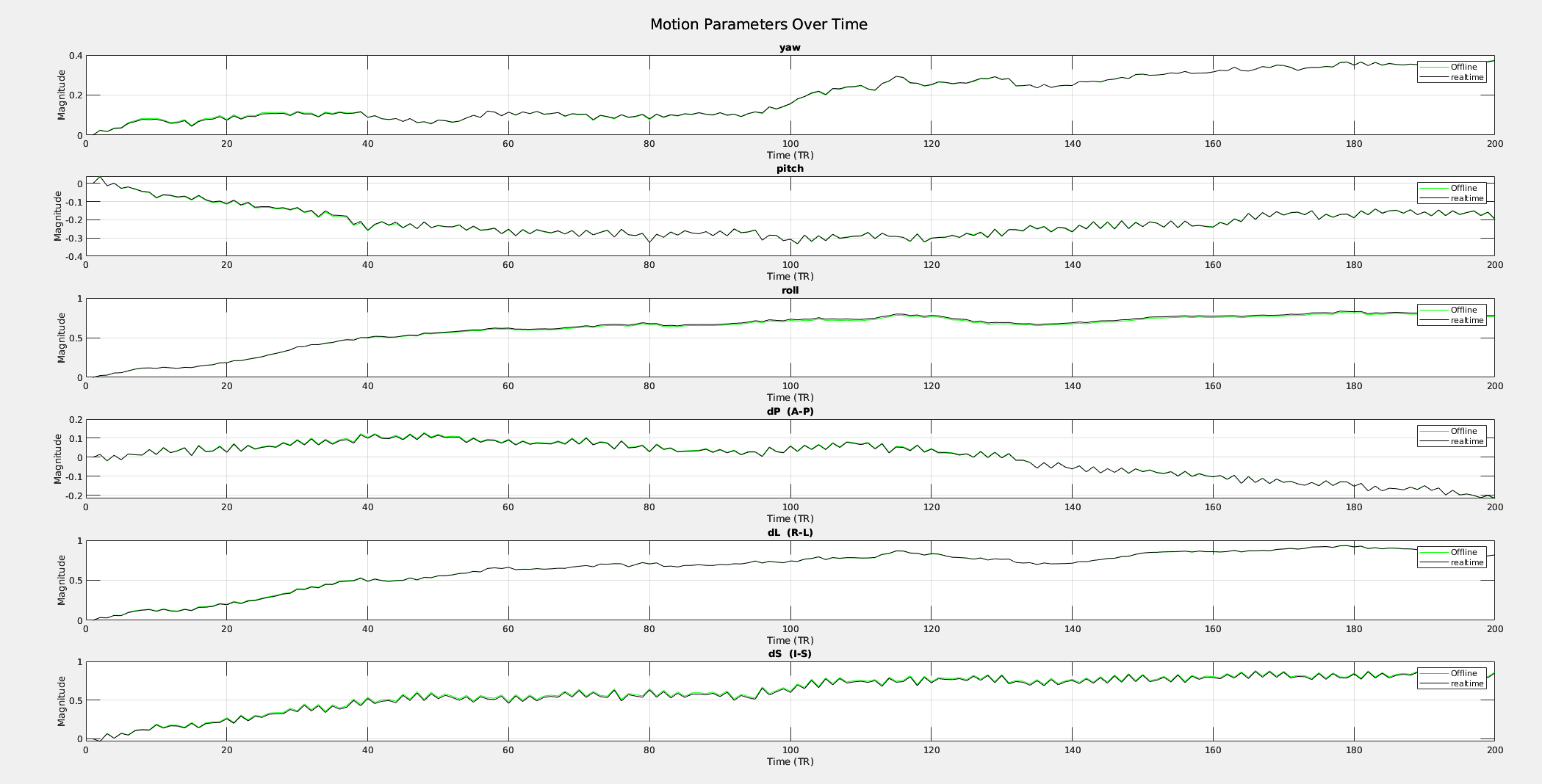
The figure, I plotted in Matlab takes the same order as the realtime graph. The black curves are from the real-time processing. Big trends and moves happen at the same time, but not always in the same direction and not with the same amplitude.

Is there a way to get my offline script closer to what realtime afni does?
I am joining as attachment, the outputs from afni, as well as the motion parameters
(I guess that the estimate from the offline is probably more exact, but I am trying to do a "calibration" for real time work so that is why I am trying to reproduce the estimate from real-time).