Large mean beta weights

AFNI version info (afni -ver):

Hi AFNI experts,

I ran a task-based fMRI until the 2d level analysis, and saved masks of interest. Then, I wanted to extract the beta weights from these masks from the first level model, for each subject to plot the corresponding values. I used 3dmaskeave on the stat file of interest specifying the sub-brik of interest (Coef). The values for specific subjects look abnormally large depending on the condition and I don't really understand why. Please, see attached. Is there an issue there? Should the beta weights be between -1 and 1? If so, why do I have such large values?

Any help would be appreciated.

Thanks,
Sarah.

Hi, Sarah-

That is indeed a nice thing to check, and a raison d'etre for emphasizing looking beyond just statistics).

In terms of what is happening here, I will assume that you used the "scale" block in afni_proc.py?

Secondly, did you look at the beta weight maps of some of those more outlying subjects---how do those look? The APQC HTML would help browse some of those quickly.

Some things that could be happening, so more of a list of possible quality control (QC) background items to investigate (which you might have done already):

  • how noisy/artifact laden did the data look? Looking at the TSNR maps and associate stats maps will help.

  • how many trial samples are there per condition? Having a very small number might make them susceptible to noise/motion spikes and contaminated estimates.

  • was alignment successful across all subjects? Depending on ROI location, there could be noisy edge bits brought in.

  • how big are some of those ROIs? If they are small, they might be ending up in a different spot.

--pt

Hi Sarah,

Would you also please show how the single subject regression model is defined? To be sure, please include whether this uses amplitude modulation.

And to be sure, are you running afni_proc.py? Optimally, it would be helpful to see the afni_proc.py command. Go ahead and focus on one subject with large values.

  • rick

Hi Ptaylor,

Thank you for your quick and helpful response. I didn’t use afni_proc.py. I know that this was suggested in a different post and will proceed with this next time, and for logistic reasons, I continue to work with the script attached.

I used meica and 3dDeconvolve.

The data looked good to me.

The task included 3 runs. The duration of each run was 9 minutes and the whole task duration was 27 minutes. Each run included 2 blocks pertaining to the predictable condition, 2 blocks pertaining to the unpredictable condition and three blocks pertaining to the no-threat condition. Each block lasted 48 seconds. The predictable block included 3 predictable cues that were presented during 8 seconds and separated by an intertrial interval that lasted between 7 and 9 seconds. 6 white noises of a duration of 40ms were presented during this block, and two aversive stimuli were administered during the onset/offset of the cue presentation.

The alignment looked good for me for all subjects included in the analyses. I removed the ones with bad alignments. I tried with different ROIs. The first approach was to use a predefined mask, a mask of the locus coeruleus. The beta weights attached before were extracted from this structure. My second approach was to extract the beta weights from a mask created via a 5-mm sphere at the peak level of clusters surviving correction at the second level. In both cases, beta weights present important variability across subjects and conditions.

I will attach some files in response to Rick below.

Thanks,
Sarah.

Hi Rick,

Thanks for your response. Please, see attached my code, including meica and the first level analysis for subject 2020. I also attached main outputs including normalized data, output from the first level, a screenshot of my GLM.

Everything looks good to me, unless you can find a big mistake in my code that I totally missed… The stats file corresponds to the t map for the “blue=unpredictable” condition.

Thank you so much again for your help.

Best,
Sarah.


Code: 
### meica
cd /data/.../nifti/
for i in `cat LIST3.txt`; do 
for j in 1 2 3; do 

cd /data/.../RUN${j}/

meica=/data/.../Workspace/me-ica/meica.py
mni=/data/.../coreg_MNI

curr_warp=$mni/.../anatQQ.sswarp_anat2mni_WARP.nii
curr_aff12_1D=$mni/.../anatQQ.sswarp_anat2mni.aff12.1D

e1=14.0
e2=37.87
e3=61.74

t1="$(ls *T1w*.nii.gz)"
dset1="$(ls *RUN${j}*e1.nii.gz)"
dset2="$(ls *RUN${j}*e2.nii.gz)"
dset3="$(ls *RUN${j}*e3.nii.gz)"

3dWarp -overwrite -quintic -deoblique -prefix anat $t1
3dWarp -overwrite -quintic -deoblique -prefix ${i}_npu${j}_e1 $dset1
3dWarp -overwrite -quintic -deoblique -prefix ${i}_npu${j}_e2 $dset2
3dWarp -overwrite -quintic -deoblique -prefix ${i}_npu${j}_e3 $dset3

python2.7 $meica --OVERWRITE -d "${i}_npu${j}_e1+orig.,${i}_npu${j}_e2+orig.,${i}_npu${j}_e3+orig." -e $e1,$e2,$e3 -a anat+orig. --mask_mode anat --coreg_mode lp-t2s --daw 10 --initcost tanh --finalcost tanh --sourceTEs -1 --cpus 15 --native --no_skullstrip  --fres=1.5

3dNwarpApply -overwrite -nwarp "$curr_warp $curr_aff12_1D" -source ${i}_npu${j}_medn_nat.nii -ainterp wsinc5 -master $mni/template/MNI2009_to_MNI+tlrc. -dxyz 1.5 -short -prefix ${i}_npu${j}_norm_1.5.nii -verb

###smooth 
norm=/data/.../DataAnalysis/native/
firstlevel=/.../first_level1.5/
for i in 2020 ; do 
for p in 1 2 3; do  
cd $norm/${i}/
cp ${i}_npu${p}_norm_1.5.nii /$firstlevel/${i}/
cd $firstlevel/${i}/
3dAutomask -prefix automask_${p} ${i}_npu${p}_norm_1.5.nii 
3dBlurInMask -input ${i}_npu${p}_norm_1.5.nii -FWHM 6 -mask automask_${p}+tlrc.HEAD -prefix ${i}_npu${p}s_norm_1.5.nii
done
done

###first level 
for i in 2020; 
do
dir=/data/.../first_level1.5/${i}
behav=/data/.../behav/${i}/
cd ${dir}
3dDeconvolve -overwrite -input ${i}_npu1s_norm_1.5.nii ${i}_npu2s_norm_1.5.nii ${i}_npu3s_norm_1.5.nii \
-polort A \
-num_stimts 11 \
-stim_times 1 ${behav}/blue_all.txt 'UBLOCK(8,1)' -stim_label 1 blue \
-stim_times 2 ${behav}/green_all.txt 'UBLOCK(8,1)' -stim_label 2 green \
-stim_times 3 ${behav}/red_all.txt 'UBLOCK(8,1)' -stim_label 3 red \
-stim_times 4 ${behav}/shockP_all.txt 'UBLOCK(2,1)' -stim_label 4 shockP \
-stim_times 5 ${behav}/shockU_all.txt 'UBLOCK(2,1)' -stim_label 5 shockU \
-stim_times 6 ${behav}/whitenoise_N_all.txt 'WAV' -stim_label 6 wn_N \
-stim_times 7 ${behav}/whitenoise_P_all.txt 'WAV' -stim_label 7 wn_P \
-stim_times 8 ${behav}/whitenoise_U_all.txt 'WAV' -stim_label 8 wn_U \
-stim_times 9 ${behav}/iti_blue_all.txt 'UBLOCK(8,1)' -stim_label 9 iti_blue \
-stim_times 10 ${behav}/iti_green_all.txt 'UBLOCK(8,1)' -stim_label 10 iti_green \
-stim_times 11 ${behav}/iti_red_all.txt 'UBLOCK(8,1)' -stim_label 11 iti_red \
-num_glt 13 \
-gltsym 'SYM: -1*green +1*red' -glt_label 1 red-green \
-gltsym 'SYM: -1*green +1*blue' -glt_label 2 blue-green \
-gltsym 'SYM: +1*red -1*blue' -glt_label 3 red-blue \
-gltsym 'SYM: +1*red +1*blue -2*green' -glt_label 4 redblue-green \
-gltsym 'SYM: +1*shockP -1*shockU' -glt_label 5 shockP-U \
-gltsym 'SYM: +1*shockP +1*shockU' -glt_label 6 shockP+U \
-gltsym 'SYM: +1*wn_P -1*wn_N' -glt_label 7 wn_P-N \
-gltsym 'SYM: +1*wn_U -1*wn_N' -glt_label 8 wn_U-N \
-gltsym 'SYM: +1*wn_P +1*wn_U -2*wn_N' -glt_label 9 wn_PU-N \
-gltsym 'SYM: -1*iti_green +1*iti_red' -glt_label 10 iti_red-green \
-gltsym 'SYM: -1*iti_green +1*iti_blue' -glt_label 11 iti_blue-green \
-gltsym 'SYM: +1*iti_red -1*iti_blue' -glt_label 12 iti_red-blue \
-gltsym 'SYM: +1*iti_red +1*iti_blue -2*iti_green' -glt_label 13 iti_redblue-green \
-tout \
-xjpeg glm_matrix.jpg \
-fitts fitts \
-errts errts \
-bucket ${i}_stats
done 

Hi, Sarah-

OK, thanks for that description. Just to note, afni_proc.py can include meica (both the older Kundu et al. code and the newer tedana one from DuPre et al.; for example, see here), and of course 3dDeconvolve.

But also a question: how did you scale your BOLD time series, so that you could interpret the coefficient values as BOLD % signal change? Was each time series scaled by its own mean?

--pt

Hi Paul,

Thanks. I am sorry, but I am not sure I understand the question. When and how am I supposed to scale my BOLD time series? I don't think I included this step in my analyses.

Best,
Sarah.

Also, if this might help, my stimulus timing files are included in txt files as follow:

157 171.99 189.01 305.99 321 337
8.0059 25.002 40.997 452 469 484.99
157 171.99 189.01 305.99 321 337

This is a txt file for one condition (in my example, the blue condition; 3 runs; 1 run per row).

Hi-

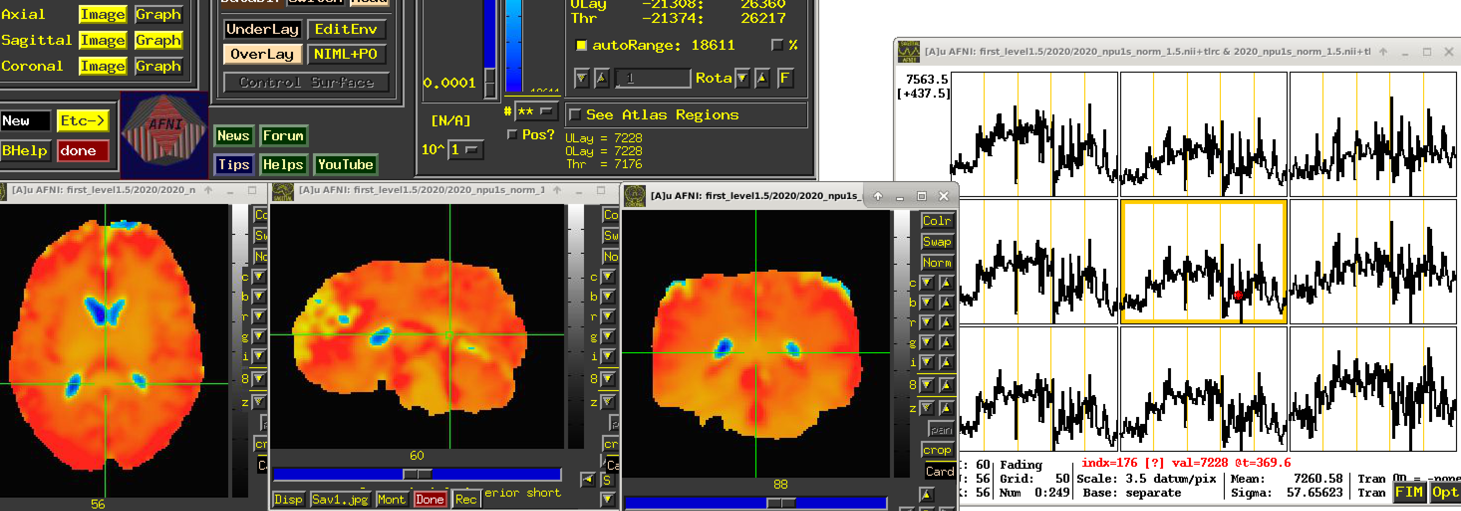
The EPI data acquired on MRI scanners for FMRI studies does not have meaningful, interpretable units. It is merely a blood oxygenation level dependent (BOLD) signal whose changes we can see over time, and does not have inherent physical interpretation. Even on the same scanner, different subjects' BOLD time series might have very different numerical baseline values, and we cannot directly compare values across them---a value of "500" has no inherent meaning, because the baseline for one subject might be 1000 and for another 478, and that 500 represents something pretty different in each case.

Consider a regression model:

y= \beta_0 + \beta_1 x_1 +\beta_2 x_2+ ... \epsilon

where y is the input data, each x_i is a regressor we put in and each \beta_i is the associated coefficient that we will solve for in the model (and the \epsilon is the residuals or leftover stuff from the input that wasn't fit by the combo of regressors); when we solve the GLM we get a set of estimated coefficient values, \hat{\beta}_i and for each one an associated statistic, t_i (which is essentially a number that says how many standard errors \sigma_i = \hat{\beta}_i/t_i the signal is away from zero).

From a "units" point of view, each \beta_i (or equivalently \hat{\beta}_i) will have units that are the ratio: (the units of y)/(the units of x_i). So, if y has arbitrary BOLD units, then the coefficient/weight will have that arbitrary unit in the numerator, too. This would mean that the overall units of the coefficient would not be easily interpretable or comparable across subjects (and probably not even across the brain).

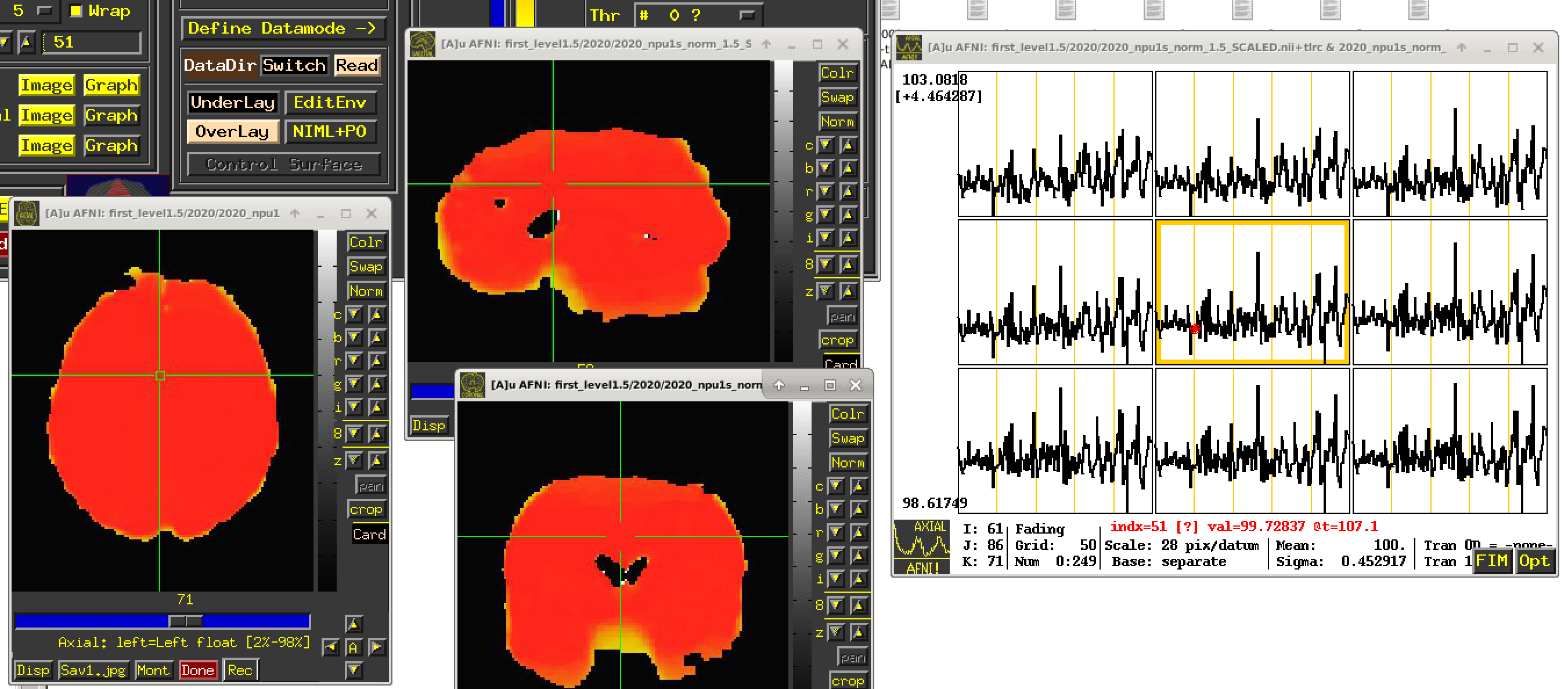
To avoid this scenario, we typically suggest that the BOLD time series should be scaled at each voxel to have meaningful units of "BOLD percent signal change". That is what the inclusion of the "scale" block in afni_proc.py will accomplish. Each voxel is scaled by its own mean to have a mean value of 100, and the fluctuations represent percent changes; so, now, seeing a value of "102" in a subject would be easily interpretable as having a 2% BOLD increase. This is described more in this paper (esp. section [C-3] Presenting results: including the effect estimates.):

and also the case of why this is generally important for the field to appropriately scale data and report/show those values here (note that different software have different default scalings, and so knowing what each one does is important; again, it is hard not to see how local/voxelwise scaling is most appropriate for FMRI):

So, the TL;DR: if you haven't scaled your data as part of processing prior to regression, the coefficients won't have interpretable units. Using afni_proc.py would help do this directly with processing, by including the scale block, which is in many of the examples.

--pt

Hi Paul,

Thank you very much for such a detailed explanation, I am learning so much right now. I wish I could have posted my questions earlier and not after a few years using afni as I am really learning a lot with your resources.

First of all - lesson learned - I will definitely use afni_proc.py in the future. Because I spent several months working on these data, and used a lot of resources on my server, I am wondering if I can solve this scaling issue without re-analyzing all my data. Is it possible?

After reading your papers, and learning more about scaling, I also came across this resource: https://andysbrainbook.readthedocs.io/en/latest/AFNI/AFNI_Short_Course/AFNI_Preprocessing/06_AFNI_Masking_Scaling.html and ran this code after the smoothing and before the first level for one of my subject (subject 2020):

I can see now, that indeed, the time series have been scaled. Please, see attached a screenshot of my subject before scaling and another one after scaling. I want to be sure that I am doing things correctly, so I have a few more questions:

  • Is this method used above a good alternative method to the afni_proc.py?
  • I used a mask of the group in my code, is that appropriate?
  • Can I use the SCALED output for the first level analysis moving forward?
### Scaling 
norm=/data/.../DataAnalysis/native/
firstlevel=/.../first_level1.5/
mask=/…/masks/
for i in 2020 ; do 
for p in 1 2 3; do 
3dTstat -prefix rm.mean_r${p}run+tlrc ${i}_npu${p}s_norm_1.5.nii
3dcalc -a ${i}_npu${p}s_norm_1.5.nii -b rm.mean_r${p}run+tlrc \
       -c $mask/mask_group.nii \
       -expr 'c * min(200, a/b*100)*step(a)*step(b)' \
       -prefix ${i}_npu${p}s_norm_1.5_SCALED.nii
done 
done

Thank you so much again for your help and time! Best, Sarah.


Hi Sarah,

That scaling is not an alternative to afni_proc.py, it is exactly the same. Looking at Andy's link, the code is a copy-and-paste from a proc script generated by afni_proc.py.

In a situation like this, I would highly recommend running afni_proc.py on at least 1 or 2 subjects and comparing the results with yours. That would have made the scaling clear, for example. Also, your results will probably be more blurry, since you are not concatenating spatial transformations. Either way, try to duplicate the regression options with an afni_proc.py example and using the @SSwarper transformation (that you seem to be doing). If there is some other peculiarity in there, it would be better to catch it before trying to publish.

  • rick

Hi Rick and Paul,

Rick, thanks for the suggestion. I re-ran my analyses using the "scaling code" above (without the -c line) and it looked like it worked. The values now look like this (see attached). Interestingly, when plotting the data the activation and graphs look the same as with the previous values. However, the correlations with some of the clinical data are gone now. I am going to run afni_proc.py on one subject, as this discussion makes me anxious. I will keep you posted if anything very different is observed.

Thank you so much for your tremendous help.

Best,
Sarah.

Hi Sarah,

Indeed, the plot of a scaled run should look exactly the same, except that the box it is plotted in has changed range to something that should hover around 100 (rather than around 7000). I am surprised to hear of correlation differences though. This should not have a very big effect on them.

If you have questions about setting up a corresponding afni_proc.py command, please let us know.

  • rick

Dear Rick and Paul,

After several discussions with team and colleagues, we believed it was worth running tedana with afni_proc.py. I successfully created a script with the help of a colleague, and while it ran very well overall, I am having one error message when trying to apply the -volreg_warp_dxyz 1.5 option. Basically, when I am adding -volreg_warp_dxyz 1.5 option; the script fails and I get this error:
3dcopy tedana_r01/TED.r01/dn_ts_OC.nii pb04.1001.r01.combine
++ 3dcopy: AFNI version=AFNI_23.2.08 (Aug 22 2023) [64-bit]
** FATAL ERROR: no datasets found!

But if I remove it, then the script is running correctly which makes me think that something is wrong with my script. If you could help me with this I would greatly appreciate it! Thank you so much again for your help so far!

###
afni_proc.py \
-subj_id ${subj_id} \
-script $data_root/${subj_id}/proc.${subj_id}.npu.csh \
-scr_overwrite \
-copy_anat $anat/anatSS.${subj_id}.nii \
-anat_has_skull no \
-anat_follower anat_w_skull anat $data_root/${subj_id}/T1w_BIC7T_${subj_id}.nii      \
-dsets_me_run $data_root/${subj_id}/${subj_id}_npu1_e?.nii \
-dsets_me_run $data_root/${subj_id}/${subj_id}_npu2_e?.nii \
-dsets_me_run $data_root/${subj_id}/${subj_id}_npu3_e?.nii \
-blocks despike tshift align tlrc volreg mask combine blur scale regress \
-radial_correlate_blocks  tcat volreg \
-tcat_remove_first_trs 2 \
-align_opts_aea  -cost lpc+ZZ \
                 -giant_move \
                 -check_flip \
-tlrc_base       $dir_MNI/MNI152_2009_template_SSW.nii.gz \
-tlrc_NL_warp \
-tlrc_NL_warped_dsets \
\
SSwarper/o.aw_${subj_id}/anatQQ.${subj_id}.nii \
SSwarper/o.aw_${subj_id}/anatQQ.${subj_id}.aff12.1D \
SSwarper/o.aw_${subj_id}/anatQQ.${subj_id}_WARP.nii \
\
-volreg_align_to MIN_OUTLIER \
-volreg_align_e2a \
-volreg_tlrc_warp \
-volreg_warp_dxyz 1.5 \
-volreg_compute_tsnr yes \
-mask_epi_anat yes \
\
-echo_times 8.5 23.17 37.84 52.51 \
-combine_method tedana \
-reg_echo 2 \
-blur_in_mask yes \
-blur_size 6 \
-regress_stim_times \
\
$data_root/${subj_id}/stimtimes/green_all.txt \
$data_root/${subj_id}/stimtimes/red_all.txt \
$data_root/${subj_id}/stimtimes/blue_all.txt \
$data_root/${subj_id}/stimtimes/iti_green_all.txt \
$data_root/${subj_id}/stimtimes/iti_blue_all.txt \
$data_root/${subj_id}/stimtimes/iti_red_all.txt \
$data_root/${subj_id}/stimtimes/shockP_all.txt \
$data_root/${subj_id}/stimtimes/shockU_all.txt \
$data_root/${subj_id}/stimtimes/whitenoise_N_all.txt \
$data_root/${subj_id}/stimtimes/whitenoise_P_all.txt \
$data_root/${subj_id}/stimtimes/whitenoise_U_all.txt \
\
-regress_stim_labels \
CUE_N \
CUE_P \
CUE_U \
ITI_N \
ITI_P \
ITI_U \
SHOCK_P \
SHOCK_U \
WN_N \
WN_P \
WN_U \
\
-regress_basis_multi \
'UBLOCK(8,1)' \
'UBLOCK(8,1)' \
'UBLOCK(8,1)' \
'UBLOCK(8,1)' \
'UBLOCK(8,1)' \
'UBLOCK(8,1)' \
'UBLOCK(2,1)' \
'UBLOCK(2,1)' \
'WAV' \
'WAV' \
'WAV' \
\
-regress_opts_3dD -num_glt 13 \
	          -gltsym 'SYM: -1*CUE_N +1*CUE_P'  \
	          -glt_label 1 CUE_P-N \
	          -gltsym 'SYM: -1*CUE_N +1*CUE_U' \
                  -glt_label 2 CUE_U-N \
                  -gltsym 'SYM: +1*CUE_U -1*CUE_P' \
                  -glt_label 3 CUE_U-P \
                  -gltsym 'SYM: +1*CUE_P +1*CUE_U -2*CUE_N' \
                  -glt_label 4 CUE_P+U-N \
                  -gltsym 'SYM: +1*SHOCK_P -1*SHOCK_U' \
                  -glt_label 5 Shock_P-U \
                  -gltsym 'SYM: +1*SHOCK_P +1*SHOCK_U' \
                  -glt_label 6 Shock_P+U \
                  -gltsym 'SYM: +1*WN_P -1*WN_N' \
                  -glt_label 7 WN_P-N \
                  -gltsym 'SYM: +1*WN_U -1*WN_N' \
                  -glt_label 8 WN_U-N \
                  -gltsym 'SYM: +1*WN_P +1*WN_U -2*WN_N' \
                  -glt_label 9 WN_P+U-N \
                  -gltsym 'SYM: -1*ITI_P +1*ITI_U' \
                  -glt_label 10 ITI_U-P \
                  -gltsym 'SYM: -1*ITI_N +1*ITI_U' \
                  -glt_label 11 ITI_U-N \
                  -gltsym 'SYM: +1*ITI_U -1*ITI_P' \
                  -glt_label 12 ITI_U-P \
                  -gltsym 'SYM: +1*ITI_P +1*ITI_U -2*ITI_N' \
                  -glt_label 13 ITI_P+U-N \
-regress_motion_per_run \
-regress_apply_mot_types demean deriv \
-regress_censor_motion 0.5 \
-regress_censor_outliers 0.15 \
-regress_3dD_stop \
-regress_reml_exec \
-regress_compute_fitts \
-regress_make_ideal_sum sum_ideal.1D \
-regress_apply_mask \
-regress_est_blur_epits \
-regress_est_blur_errts \
-regress_run_clustsim no \
-test_stim_files no \
-html_review_style pythonic \
-execute

Blockquote

Blockquote

Howdy-

Perhaps could you please email me the full output* log text from running afni_proc.py? I wonder if something fails before that, causing the dataset to not be created, and that might clarify the actual problem. For example, perhaps tedana fails because the data is too high resolution or runs out of memory (the process gets killed). It's hard for me to see how else setting the final voxel resolution would cause an error.

(Out of curiosity, what is the input voxel resolution? If it were much larger, like 3mm isotropic, then this final output data would have nearly an order of magnitude more voxels, and hence there could be a memory issue appearing, perhaps. But this is only speculation at this point.)

thanks,
pt

Hi Paul,

Thank you for your swift response. We're working with two datasets, where the voxel resolution is 1.5 for one and 2.5 for the other. The goal is to normalize both datasets to a voxel resolution of 1.5mm. As an update, I reran the script with and without the volreg_warp_dxy.1.5 option, and unfortunately, it failed in both cases.

I'll be sending you the log text shortly for your review. Thanks again for your help!

Sarah.