Yes thank you! The experience was very good, its very useful! I think it just need to learn how check, verify "goodness of fit".
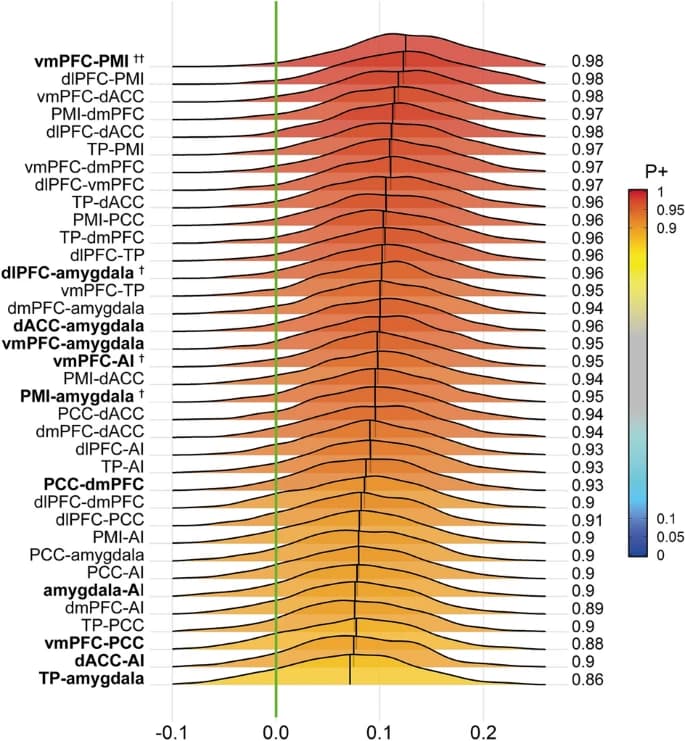
Then, you can directly access the Markov chain Monte Carlo simulation results. Utilize the functions in MBA.R in your AFNI binary directory to construct uncertainty intervals with your preferred quantile. For instance, information about region pairs can be found under the heading:
Ah, very cool! so by running the following one can access all the subthreshold details?
rp_summary <- function(ps, ns, nR) {
  mm <- apply(ps, c(2,3), mean)
  for(ii in 1:nR) for(jj in 1:nR) ps[,ii,jj] <- sqrt(2)*(ps[,ii,jj] - mm[ii,jj]) + mm[ii,jj]
  RP <- array(NA, dim=c(nR, nR, 8))
  RP[,,1] <- apply(ps, c(2,3), mean)
  RP[,,2] <- apply(ps, c(2,3), sd)
  RP[,,3] <- apply(ps, c(2,3), cnt, ns)
  RP[,,4:8] <- aperm(apply(ps, c(2,3), quantile, probs=c(0.025, 0.05, 0.5, 0.95, 0.975)), dim=c(2,3,1))
  dimnames(RP)[[1]] <- dimnames(ps)[[2]]
  dimnames(RP)[[2]] <- dimnames(ps)[[3]]
  dimnames(RP)[[3]] <- c('mean', 'SD', 'P+', '2.5%', '5%', '50%', '95%', '97.5%')
  return(RP)
}

# extract region-pair posterior samples for an effect 'tm'
region_pair <- function(pe, ge, tm, nR) {
  ps0 <- array(apply(ge[['mmROI1ROI2']][,,tm], 2, "+", ge[['mmROI1ROI2']][,,tm]), c(ns, nR, nR)) # obtain (ROIi, ROIj) matrix for region-specific main effects
  ps <- apply(ps0, c(2,3), '+', pe[,tm]) # add the common effect to the matrix

  dimnames(ps) <- list(1:ns, rL, rL)
  tmp <- ps

  sel1 <- match(dimnames(ge$`ROI1:ROI2`)[[2]], outer(dimnames(ps)[[2]],dimnames(ps)[[3]], function(x,y) paste(x,y,sep="_")))
  sel2 <- match(dimnames(ge$`ROI1:ROI2`)[[2]], outer(dimnames(ps)[[2]],dimnames(ps)[[3]], function(x,y) paste(y,x,sep="_")))

  ad <- function(tt,ge,s1,s2) {tt[s1] <- tt[s1] + ge; tt[s2] <- tt[s2] + ge; return(tt)}
  for(ii in 1:ns) tmp[ii,,] <- ad(tmp[ii,,], ge$`ROI1:ROI2`[ii,,tm], sel1, sel2)  # add the interaction
  ps <- tmp
  return(ps)
}

ns <- lop$iterations*lop$chains/2
#nR <- nlevels(lop$dataTable$ROI1)
pe <- fixef(fm, summary = FALSE) # Population-Level Estimates
ge <- ranef(fm, summary = FALSE) # Extract Group-Level (or random-effect) Estimates
nR <- length(union(levels(lop$dataTable$ROI1), levels(lop$dataTable$ROI2)))
if(!is.na(lop$ROIlist)) {
   lop$ROI$order <- as.character(lop$ROI$order)
   if(!setequal(lop$ROI$order, union(levels(lop$dataTable$ROI1), levels(lop$dataTable$ROI2))))
   errex.AFNI(paste("The ROIs listed under option -ROIlist do not fully match those specified in the data table!"))
   # change the factor levels to characters
}

rp_summary(region_pair(pe, ge, lop$EOIq[ii], nR), ns, nR)
You can find an R plot function here. Simply provide the posterior samples as input in the format of the data.frame dat .
Hm... so that would the output of the region_summary function right?
glimpse(region_pair(pe, ge, lop$EOIq[ii], nR))
 num [1:2000, 1:8, 1:8] 0.05109 0.00483 -0.0305 -0.05837 -0.00657 ...
 - attr(*, "dimnames")=List of 3
  ..$ : chr [1:2000] "1" "2" "3" "4" ...
  ..$ : chr [1:8] "CA1" "CA2" "CA3" "CA4" ...
  ..$ : chr [1:8] "CA1" "CA2" "CA3" "CA4" ...
but it will have to be altered so as to only include unique pairwise combination of N rois right? I basically need to select the "upper triangle" of the NxNx2000 matrix?
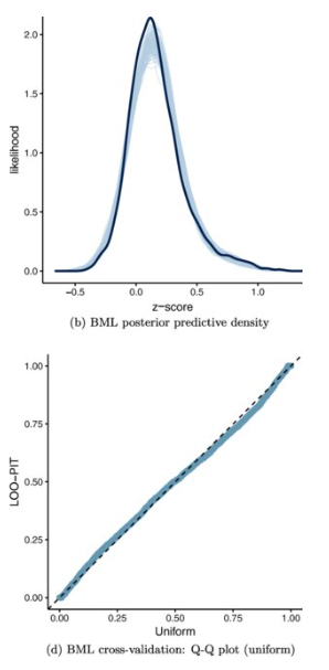
Could you illustrate how one ought to do the posterior predictive checks?