Enhancing HDR Detection Sensitivity through Profile Estimation
Gang Chen
Preface
The hemodynamic response (HDR) exhibits a distinctive profile characterized by an initial dip, an overshoot, and an undershoot. This profile is well-known in the field of neuroimaging (shown in the left figure) and is commonly represented by a canonical function (shown in the right figure). The canonical function serves as an impulse curve in individual-level data analysis, and its adoption has contributed to its widespread familiarity among researchers.


The canonical HDR function is a valuable tool that plays a crucial role in the modeling process. By transforming the complex 1D curve of the HDR into a standardized profile, it serves as a data reduction technique. The application of the canonical function allows us to characterize the HDR in response to a task condition with a scalar value that represents the magnitude of the effect. This simplification greatly facilitates subsequent analyses, such as population-level analysis, statistical learning, and classifications, making them more convenient and manageable.
However, this simplification comes at a significant cost. The use of a canonical HDR function restricts flexibility and fails to account for shape variations. Consequently, this inflexibility can result in under-fitting, compromised detection sensitivity, and impaired reproducibility.
A wide range of methodologies exist in improving HDR estimation. Here, we specifically focus on a particular data-driven approach of condition-level HDR estimation elucidated in a recent publication:
Chen, G., Taylor, P.A., Reynolds, R.C., Leibenluft, E., Pine, D.S., Brotman, M.A., Pagliaccio, D., Haller, S.P., 2023. BOLD Response is more than just magnitude: Improving detection sensitivity through capturing hemodynamic profiles. NeuroImage 277, 120224.
Briefly, the individual-level estimation of HDR involves the use of splines, such as tents and cubic splines in AFNI or FIR in FSL/SPM. Subsequently, the estimated HDR at consecutive time points is carried over to the population level, where it is fitted with smooth splines. To enhance predictive accuracy, a regularization process is implemented, penalizing the roughness of the HDR profile.
Prerequisites in experimental design
Experimental design is a crucial component in statistical modeling, particularly in HDR estimation. We emphasize the following two aspects:
-
To achieve proper estimation efficiency, it is critical to incorporate inter-stimulus jittering and randomize trial sequences across conditions.
-
A short TR (e.g., 2 s or less) is required to achieve a proper accuracy in estimating HDR profiles. If adopting a short TR is challenging, varying stimulus timing among participants can be considered. For example, with a TR of 2 seconds, HDR samples can be collected at the TR grids for half of the participants, while obtaining shifted samples by half a TR (i.e., 1 second) for the other half. This approach allows for HDR estimation at a finer temporal resolution of 1 second at the population level.
Individual-level modeling strategy
The choice of HDR duration is a critical decision in HDR estimation. A duration that is too short may result in a loss of accuracy in capturing the slow recovery phase, while an excessively long duration can lead to inefficiency and the potential risk of collinearity. For event-related designs, it is advisable to consider durations within the range of 16 to 20 seconds.
Estimating the HDR at the individual level is achieved through a deconvolution process. To illustrate how to specify a chosen spline type, let's consider a concrete example using AFNI. Suppose we want to cover an HDR duration of 16 s for a task condition with a TR of 2 s. In the 3dDeconvolve command, we can use the following specification:
TENT(2,16,8)
Here's how the three parameters, 2, 16, and 8, work:
(1) No response is assumed at the stimulus onset (0 s) and at the end (18 s).
(2) The HDR is estimated at 8 TRs (spline knots) that cover the period from 2 to 16 s.
Some specification variations are worth mentioning. If one wants to capture the HDR at the stimulus onset, use the following specification in 3dDeconvolve :
TENT(0,16,9)
Similarly, if one assumes that the HDR starts one TR ahead of the stimulus onset, use:
TENT(-2,16,10)
These variations allow one to adjust the timing of the HDR estimation to capture the desired response.
How to estimate HDRs in a higher time resolution than the TR permits? For those who are adventurous, an alternative experiment design can be considered based on the approach discussed in the previous section. In this design, half of the participants perform the task at the TR grids, while the other half's stimulus onset is shifted by half TR.
For the first half of participants, their HDRs can be specified as usual using, for example, the following specification in 3dDeconvolve:
TENT(2,16,8)
These HDRs are estimated at the TR grids: 2, 4, ..., 16 s.
For the second half of participants, artificially subtract their real stimulus onset by half TR. In the words, move their stimulus onset backward by half TR during modeling so that their stimulus onset is aligned with the TR grids. The same specification as the first half participants can then be used:
TENT(2,16,8)
As a result, the sampled HDRs for these second half participants would actually be sampled at 1, 3, ..., 15 s. The ultimate goal of this approach is to estimate HDRs with higher accuracy by using samples available from every half TR instead of the usual TR resolution.
Population-level HDR estimation using smooth splines
One distinguishing aspect of our approach to population-level HDR estimation is the incorporation of a roughness penalty. This regularization constraint imposes a requirement for smoothness in the estimated HDR profiles. While this smoothness contributes to visual appeal, its primary significance lies in its alignment with the underlying physiological mechanism and its potential to enhance predictive accuracy. By enforcing a smoothness constraint, the approach captures the inherent coherence and temporal dynamics of the HDR, leading to more accurate and reliable estimation outcomes.
The program 3dMSS in AFNI conducts population-level HDR estimation utilizing smooth splines. To provide a practical illustration, we present a demonstrative example from our recent publication.
(1) HDR comparison between two groups
The script below showcases a comparison of HDRs between two groups: BP (individuals with bipolar disorder) and HV (healthy volunteers) at the population level. Each individual-level HDR is characterized by 14 time points, with a time resolution of TR = 1.25s. Additionally, two covariates, namely sex and age, are taken into consideration during the analysis.
3dMSS -prefix output -jobs 16             \
      -lme 'sex+age+s(TR)+s(TR,by=group)' \
      -ranEff 'list(subject=~1)'          \
      -qVars 'sex,age,TR,group'           \
      -prediction @HDR.table              \
      -dataTable  @data.table
The details of the aforementioned script are explained as follows. The output filename and the number of CPUs for parallelization are specified using the -prefix and -jobs options, respectively. In the model specification indicator -lme , the expression s() represents the smooth function. The terms s(TR) and s(TR,by=group) encode the overall HDR profile and the HDR difference between the two groups, respectively. Under the -ranEff option, the term list(subject=~1) denotes the participant-specific effects that account for cross-individual variability in the intercept. The default number of thin plate splines, K = 10, is set. The -qVars option identifies the quantitative variables, which, in this case, include TR, age, as well as dummy-coded sex and group. Lastly, the -prediction and -dataTable specifiers refer to the table for HDR prediction and the table containing input data information, respectively. The input file, "data.table," is structured in the form of a long data frame:
subject age sex group TR  InputFile
s1      29   1    1   0   s1.Inc.b0.nii
s1      29   1    1   1   s1.Inc.b1.nii
s1      29   1    1   2   s1.Inc.b2.nii
s1      29   1    1   3   s1.Inc.b3.nii
s1      29   1    1   4   s1.Inc.b4.nii
...
The input file "HDR.table" contains the table used for predicted HDRs and is shown below. In this table, special attention should be given to the time incremental size, which is set to 0.25 s in the last column. This setting enables the predicted HDRs to be displayed in a high temporal resolution.
label       age    sex   group   TR
group1      20     0     1    0.00
group1      20     0     1    0.25
group1      20     0     1    0.50
...
group2      20     0    -1    0.00
group2      20     0    -1    0.25
group2      20     0    -1    0.50
...
Note:
- The covariates
ageandsexare set to their respective centered values. - The
groupvariable is coded using each group's specific numerical value. - The
TR(time resolution) is set to a small value to allow smooth visualization of the predicted profiles.
Big effort yields big rewards. It is gratifying to see the enhanced detection sensitivity offered by the data-driven approach of HDR estimation (shown on the right, below) when compared to the canonical approach (shown on the left, below).
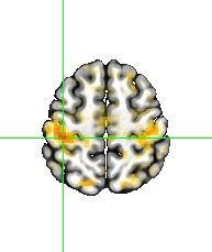
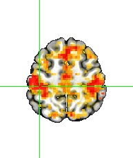
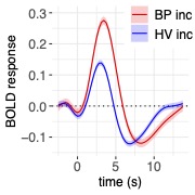
One final point to consider is that scientific investigations should place greater emphasis on effect estimation rather than making decisions solely based on statistical evidence. In other words, it is more important to focus on pursuing predictive accuracy and precision rather than relying on a dichotomous decision. For this reason, the results presented in the above figure are not subjected to artificial thresholding/clustering but are presented in a gradual manner as proposed in previous publications (e.g., here and here). The predicted HDRs in the 3dMSS output can be used for visualization and verification of the presence of HDR in a brain response. The power of visual examination should not be underestimated, as it allows for a comprehensive comparison of accuracy and the amount of information provided. In this regard, comparing the 1D curve obtained from HDR estimation (shown on the right, above) to a single scalar in the canonical approach (shown on the left, above) highlights the advantages of the former in terms of accuracy, richness, and detailed representation.
(2) HDR assessment for one group
The script below illustrates the assessment of HDRs for one group of participants: BP (individuals with bipolar disorder) at the population level. Each individual-level HDR is characterized by 14 time points, with a time resolution of TR = 1.25s. Additionally, two covariates, namely sex and age, are taken into consideration during the analysis.
3dMSS -prefix output -jobs 16             \
      -lme 'sex+age+s(TR)' \
      -ranEff 'list(subject=~1)'          \
      -qVars 'sex,age,TR,group'           \
      -prediction @HDR.table              \
      -dataTable  @data.table
(3) HDR contrast between two task conditions
In this case, obtain the contrast between the two conditions at each time point at the individual level. Then, adopt the same scripting strategy as in (2). We suggestion that each condition is also analyzed separately so that the condition-level HDRs can be compared with their contrast at the population level.
Conclusion
It is expected that information loss occurs when the hemodynamic response is represented by and reduced to a scalar for a canonical curve. However, despite the higher model complexity and computational cost, it is worthwhile to make the extra effort to minimize information loss and enhance detection sensitivity. We believe that HDR estimation through smooth splines provides a valuable tool for improving reproducibility in neuroimaging data analysis.